- 入门教程
- ANN教程
- CNN教程
- RNN教程
 《TensorFlow入门教程》
 关注我们

TensorFlow - 感知器的隐藏层

在本章中,无涯教程将专注于从x和f(x)的已知点集中学习的网络,由单个隐藏层将构建此简单网络。
解释感知器隐藏层的代码如下所示-
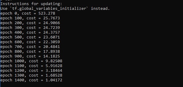
#Importing the necessary modules
import tensorflow as tf
import numpy as np
import math, random
import matplotlib.pyplot as plt

np.random.seed(1000)
function_to_learn=lambda x: np.cos(x) + 0.1*np.random.randn(*x.shape)
layer_1_neurons=10
NUM_points=1000

#训练参数
batch_size=100
NUM_EPOCHS=1500

all_x=np.float32(np.random.uniform(-2*math.pi, 2*math.pi, (1, NUM_points))).T
   np.random.shuffle(all_x)

train_size=int(900)
#训练给定集合中的前 700 个点 x_training=all_x[:train_size]
y_training=function_to_learn(x_training)

#训练给定集合中的最后 300 个点 x_validation=all_x[train_size:]
y_validation=function_to_learn(x_validation)

plt.figure(1)
plt.scatter(x_training, y_training, c='blue', label='train')
plt.scatter(x_validation, y_validation, c='pink', label='validation')
plt.legend()
plt.show()

X=tf.placeholder(tf.float32, [None, 1], name="X")
Y=tf.placeholder(tf.float32, [None, 1], name="Y")

#first layer
#神经元数=10
w_h=tf.Variable(
   tf.random_uniform([1, layer_1_neurons],\minval=-1, maxval=1, dtype=tf.float32))
b_h=tf.Variable(tf.zeros([1, layer_1_neurons], dtype=tf.float32))
h=tf.nn.sigmoid(tf.matmul(X, w_h) + b_h)

#output layer
#Number of neurons=10
w_o=tf.Variable(
   tf.random_uniform([layer_1_neurons, 1],\minval=-1, maxval=1, dtype=tf.float32))
b_o=tf.Variable(tf.zeros([1, 1], dtype=tf.float32))

#建立模型
model=tf.matmul(h, w_o) + b_o

#最小化成本函数(模型 - Y)
train_op=tf.train.AdamOptimizer().minimize(tf.nn.l2_loss(model - Y))

#开始学习阶段
sess=tf.Session() sess.run(tf.initialize_all_variables())

errors=[]
for i in range(NUM_EPOCHS):
   for start, end in zip(range(0, len(x_training), batch_size),\
      range(batch_size, len(x_training), batch_size)):
      sess.run(train_op, feed_dict={X: x_training[start:end],\Y: y_training[start:end]})
   cost=sess.run(tf.nn.l2_loss(model - y_validation),\feed_dict={X:x_validation})
   errors.append(cost)

   if i%100 == 0:
      print("epoch %d, cost=%g" % (i, cost))

plt.plot(errors,label='MLP Function Approximation') plt.xlabel('epochs')
plt.ylabel('cost')
plt.legend()
plt.show()
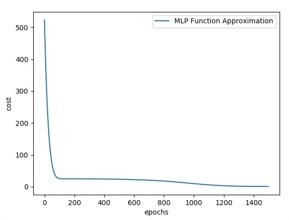
以下是功能层近似的表示-
来源:LearnFk无涯教程网
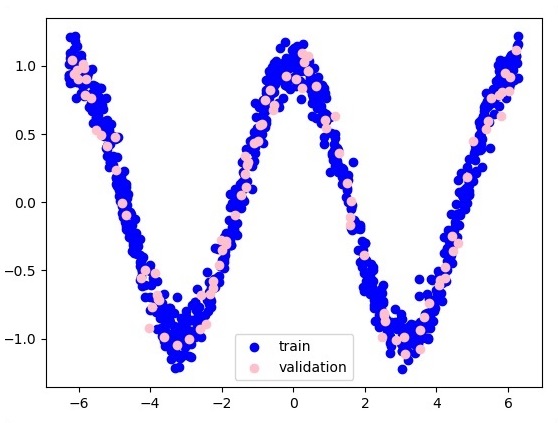
这里,两个数据以W的形式表示。两个数据是:训练和验证,它们以不同的颜色表示,如在图例部分中可见。
祝学习愉快!(内容编辑有误?请选中要编辑内容 -> 右键 -> 修改 -> 提交!)
Spring Cloud 微服务项目实战 -〔姚秋辰(姚半仙)〕
好记忆不如烂笔头。留下您的足迹吧 :)