本文实现两个分类器: softmax分类器和感知机分类器
Softmax分类器
Softmax分类是一种常用的多类别分类算法,它可以将输入数据映射到一个概率分布上。Softmax分类首先将输入数据通过线性变换得到一个向量,然后将向量中的每个元素进行指数函数运算,最后将指数运算结果归一化得到一个概率分布。这个概率分布可以被解释为每个类别的概率估计。
定义
定义一个softmax分类器类:
class SoftmaxClassifier(nn.Module):
    def __init__(self,input_size,output_size):
        # 调用父类的__init__()方法进行初始化
        super(SoftmaxClassifier,self).__init__()
        # 定义一个nn.Linear对象,用于将输入特征映射到输出类别
        self.linear = nn.Linear(input_size,output_size)

    def forward(self,x):
        x = self.linear(x) # 传递给线性层
        return nn.functional.softmax(x,dim=1) # 得到概率分布

    def compute_accuracy(self,output,labels):
        preds = torch.argmax(output,dim=1) # 获取每个样本的预测标签
        correct = torch.sum(preds == labels).item() # 计算正确预测的数量
        accuracy = correct / len(labels) # 除以总样本数得到准确率
        return accuracy
如上定义三个方法:
-
__init__(self):构造函数,在类初始化时运行,调用父类的__init__()方法进行初始化 -
forward(self):模型前向计算过程 -
compute_accuracy(self):计算模型的预测准确率
训练
生成训练数据:
import numpy as np

# 生成随机样本(包含训练数据和测试数据)
def generate_rand_samples(dot_num=100):
    x_p = np.random.normal(3., 1, dot_num)
    y_p = np.random.normal(3., 1, dot_num)
    y = np.zeros(dot_num)
    C1 = np.array([x_p, y_p, y]).T
    x_n = np.random.normal(7., 1, dot_num)
    y_n = np.random.normal(7., 1, dot_num)
    y = np.ones(dot_num)
    C2 = np.array([x_n, y_n, y]).T
    x_n = np.random.normal(3., 1, dot_num)
    y_n = np.random.normal(7., 1, dot_num)
    y = np.ones(dot_num)*2
    C3 = np.array([x_n, y_n, y]).T
    x_n = np.random.normal(7, 1, dot_num)
    y_n = np.random.normal(3, 1, dot_num)
    y = np.ones(dot_num)*3
    C4 = np.array([x_n, y_n, y]).T
    data_set = np.concatenate((C1, C2, C3, C4), axis=0)
    np.random.shuffle(data_set)

    return data_set[:,:2].astype(np.float32),data_set[:,2].astype(np.int32)

X_train,y_train = generate_rand_samples()
y_train[y_train == -1] = 0
设置训练前的前置参数,并初始化分类器
num_inputs = 2  # 输入维度大小
num_outputs = 4  # 输出维度大小
learning_rate = 0.01  # 学习率
num_epochs = 2000 # 训练周期数

# 归一化数据 将数据特征减去均值再除以标准差
X_train = (X_train - X_train.mean(axis=0)) / X_train.std(axis=0)
y_train = y_train.astype(np.compat.long)

# 创建model并初始化
model = SoftmaxClassifier(num_inputs, num_outputs)
criterion = nn.CrossEntropyLoss() # 交叉熵损失
optimizer = optim.SGD(model.parameters(), lr=learning_rate)  # SGD优化器
训练:
# 遍历训练周期数
for epoch in range(num_epochs):
    outputs = model(torch.tensor(X_train))  # 前向传递计算
    loss = criterion(outputs,torch.tensor(y_train))  # 计算预测输出和真实标签之间的损失
    train_accuracy = model.compute_accuracy(outputs,torch.tensor(y_train))  # 计算模型当前训练周期中准确率

    optimizer.zero_grad()  # 清楚优化器中梯度
    loss.backward()  # 计算损失对模型参数的梯度
    optimizer.step()

    # 打印信息
    if (epoch + 1) % 10 == 0:
        print(f"Epoch [{epoch+1}/{num_epochs}], Loss: {loss.item():.4f}, Accuracy: {train_accuracy:.4f}")
运行:
Epoch [1820/2000], Loss: 0.9947, Accuracy: 0.9575
Epoch [1830/2000], Loss: 0.9940, Accuracy: 0.9600
Epoch [1840/2000], Loss: 0.9932, Accuracy: 0.9600
Epoch [1850/2000], Loss: 0.9925, Accuracy: 0.9600
Epoch [1860/2000], Loss: 0.9917, Accuracy: 0.9600
....
测试
生成测试并测试:
X_test, y_test = generate_rand_samples()  # 生成测试数据
X_test = (X_test- np.mean(X_test)) / np.std(X_test)  # 归一化
y_test = y_test.astype(np.compat.long)
predicts = model(torch.tensor(X_test))  # 获取模型输出
accuracy = model.compute_accuracy(predicts,torch.tensor(y_test))  # 计算准确度
print(f'Test Accuracy: {accuracy:.4f}')
输出:
Test Accuracy: 0.9725
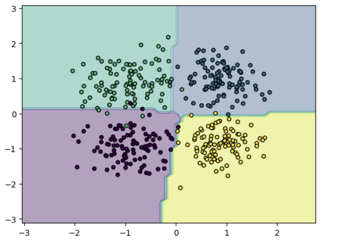
绘制图像:
# 绘制图像
x_min, x_max = X_test[:, 0].min() - 1, X_test[:, 0].max() + 1
y_min, y_max = X_test[:, 1].min() - 1, X_test[:, 1].max() + 1
xx, yy = np.meshgrid(np.arange(x_min, x_max, 0.1), np.arange(y_min, y_max, 0.1))
Z = model(torch.tensor(np.c_[xx.ravel(), yy.ravel()], dtype=torch.float32)).argmax(dim=1).numpy()
Z = Z.reshape(xx.shape)
plt.contourf(xx, yy, Z, alpha=0.4)
plt.scatter(X_test[:, 0], X_test[:, 1], c=y_test, s=20, edgecolor='k')
plt.show()
感知机分类器
实现与上述softmax分类器相似,此处实现sigmod感知机,采用sigmod作为分类函数,该函数可以将线性变换的结果映射为0到1之间的实数值,通常被用作神经网络中的激活函数
sigmoid感知机的学习算法与普通的感知机类似,也是采用随机梯度下降(SGD)的方式进行更新。不同之处在于,sigmoid感知机的输出是一个概率值,需要将其转化为类别标签。
通常使用阈值来决定输出值所属的类别,如将输出值大于0.5的样本归为正类,小于等于0.5的样本归为负类。
定义
# 感知机分类器
class PerceptronClassifier(nn.Module):
    def __init__(self, input_size,output_size):
        super(PerceptronClassifier, self).__init__()
        self.linear = nn.Linear(input_size,output_size)

    def forward(self, x):
        logits = self.linear(x)
        return torch.sigmoid(logits)

    def compute_accuracy(self, pred, target):
        pred = torch.where(pred >= 0.5, 1, -1)
        accuracy = (pred == target).sum().item() / target.size(0)
        return accuracy
给定一个输入向量(x1,x2,x3...xn),输出为y=σ(w⋅x+b)=1/(e^−(w⋅x+b))
训练
生成训练集:
def generate_rand_samples(dot_num=100):
    x_p = np.random.normal(3., 1, dot_num)
    y_p = np.random.normal(3., 1, dot_num)
    y = np.ones(dot_num)
    C1 = np.array([x_p, y_p, y]).T
    x_n = np.random.normal(6., 1, dot_num)
    y_n = np.random.normal(0., 1, dot_num)
    y = np.ones(dot_num)*-1
    C2 = np.array([x_n, y_n, y]).T
    data_set = np.concatenate((C1, C2), axis=0)
    np.random.shuffle(data_set)
    return data_set[:,:2].astype(np.float32),data_set[:,2].astype(np.int32)

X_train,y_train = generate_rand_samples()
X_test,y_test = generate_rand_samples()
该过程与上述softmax分类器相似:
num_inputs = 2
num_outputs = 1
learning_rate = 0.01
num_epochs = 200

# 归一化数据 将数据特征减去均值再除以标准差
X_train = (X_train - X_train.mean(axis=0)) / X_train.std(axis=0)

# 创建model并初始化
model = PerceptronClassifier(num_inputs, num_outputs)
optimizer = optim.SGD(model.parameters(), lr=learning_rate)  # SGD优化器

criterion = nn.functional.binary_cross_entropy
训练:
# 遍历训练周期数
for epoch in range(num_epochs):
    outputs = model(torch.tensor(X_train))
    labels = torch.tensor(y_train).unsqueeze(1)
    loss = criterion(outputs,labels.float())
    train_accuracy = model.compute_accuracy(outputs, labels)

    optimizer.zero_grad()
    loss.backward()
    optimizer.step()

    if (epoch + 1) % 10 == 0:
        print(f"Epoch [{epoch+1}/{num_epochs}], Loss: {loss.item():.4f}, Accuracy: {train_accuracy:.4f}")
输出:
Epoch [80/200], Loss: -0.5429, Accuracy: 0.9550
Epoch [90/200], Loss: -0.6235, Accuracy: 0.9550
Epoch [100/200], Loss: -0.7015, Accuracy: 0.9500
Epoch [110/200], Loss: -0.7773, Accuracy: 0.9400
....
测试
X_test, y_test = generate_rand_samples() # 生成测试集
X_test = (X_test - X_test.mean(axis=0)) / X_test.std(axis=0)

test_inputs = torch.tensor(X_test)
test_labels = torch.tensor(y_test).unsqueeze(1)
with torch.no_grad():
    outputs = model(test_inputs)
    accuracy = model.compute_accuracy(outputs, test_labels)
    print(f"Test Accuracy: {accuracy:.4f}")
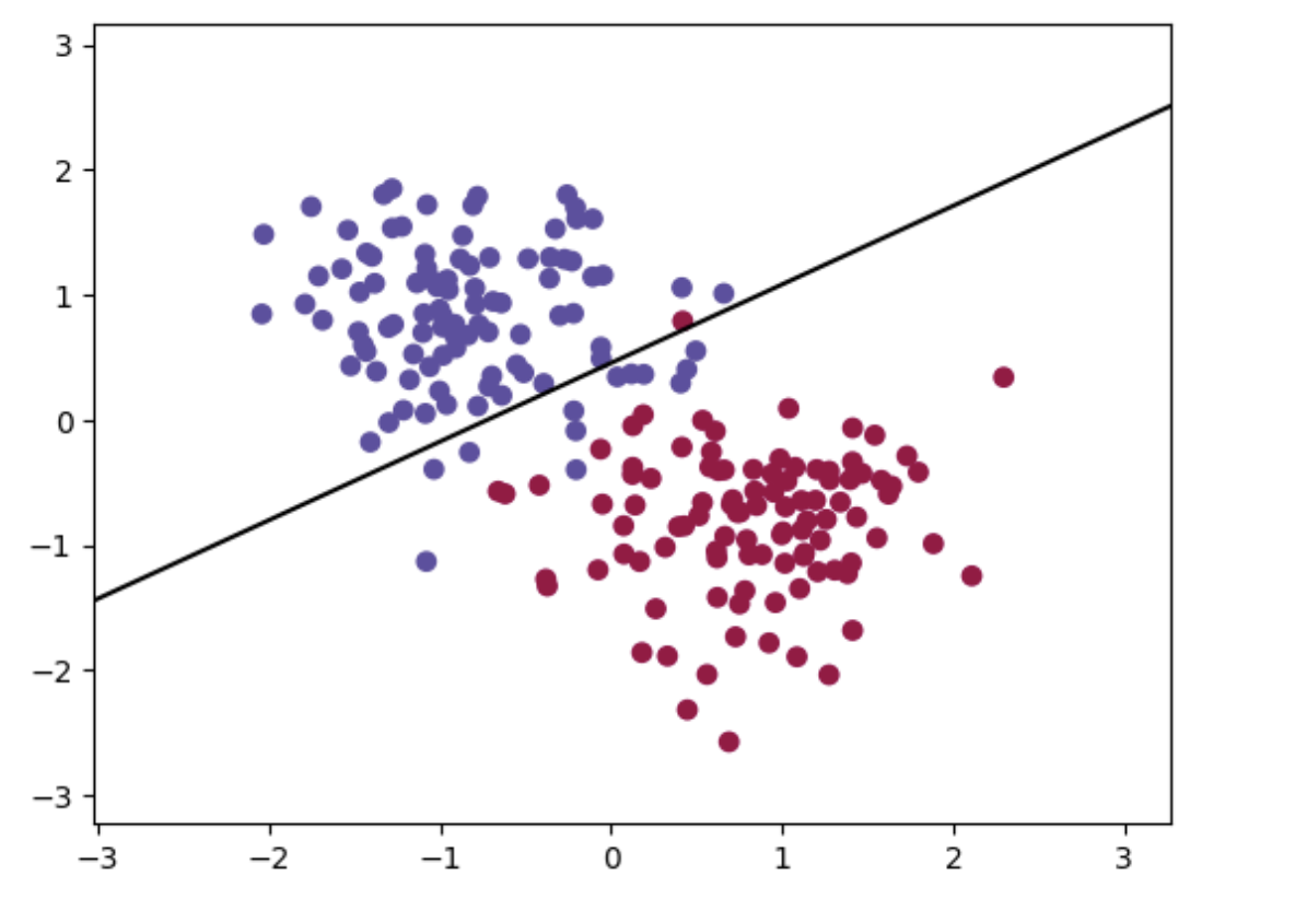
绘图:
x_min, x_max = X_test[:, 0].min() - 1, X_test[:, 0].max() + 1
y_min, y_max = X_test[:, 1].min() - 1, X_test[:, 1].max() + 1
xx, yy = torch.meshgrid(torch.linspace(x_min, x_max, 100), torch.linspace(y_min, y_max, 100))

# 预测每个点的类别
Z = torch.argmax(model(torch.cat((xx.reshape(-1,1), yy.reshape(-1,1)), 1)), 1)
Z = Z.reshape(xx.shape)

# 绘制分类图
plt.contourf(xx, yy, Z, cmap=plt.cm.Spectral,alpha=0.0)

# 绘制分界线
w = model.linear.weight.detach().numpy()  # 权重
b = model.linear.bias.detach().numpy()  # 偏置
x1 = np.linspace(x_min, x_max, 100)
x2 = (-b - w[0][0]*x1) / w[0][1]
plt.plot(x1, x2, 'k-')

# 绘制样本点
plt.scatter(X_train[:, 0], X_train[:, 1], c=y_train, cmap=plt.cm.Spectral)
plt.show()