分类算法 中的 Python实现函数

为了在Python中实现SVM，无涯教程将从标准库导入开始，如下所示-

import numpy as np
import matplotlib.pyplot as plt
from scipy import stats
import seaborn as sns; sns.set()

接下来，从sklearn.dataset.sample_generator创建具有线性可分离数据的样本数据集，以使用SVM进行分类-

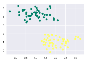
from sklearn.datasets.samples_generator import make_blobs
X, y=make_blobs(n_samples=100, centers=2, random_state=0, cluster_std=0.50)
plt.scatter(X[:, 0], X[:, 1], c=y, s=50, cmap='summer');

以下是生成具有100个样本和2个聚类的样本数据集后的输出-

知道SVM支持判别分类。它通过在二维的情况下简单地找到一条线，在多维的情况下通过歧管来简单地将类彼此划分。它在上述数据集上实现如下-

xfit = np.linspace(-1, 3.5)
plt.scatter(X[:, 0], X[:, 1], c = y, s = 50, cmap = 'summer')
plt.plot([0.6], [2.1], 'x', color = 'black', markeredgewidth = 4, markersize = 12)
for m, b in [(1, 0.65), (0.5, 1.6), (-0.2, 2.9)]:
plt.plot(xfit, m * xfit + b, '-k')
plt.xlim(-1, 3.5);

输出如下-

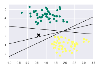
从上面的输出中可以看到，有三种不同的分隔符可以完美地区分以上示例。

正如讨论的那样，SVM的主要目标是将数据集划分为类，以找到最大的边际超平面(MMH)，而不是在类之间绘制零线，可以在每条线周围画出一定宽度的边界，直到最近的点。它可以做到如下-

xfit = np.linspace(-1, 3.5)
plt.scatter(X[:, 0], X[:, 1], c = y, s = 50, cmap = 'summer')

for m, b, d in [(1, 0.65, 0.33), (0.5, 1.6, 0.55), (-0.2, 2.9, 0.2)]:
   yfit = m * xfit + b
   plt.plot(xfit, yfit, '-k')
   plt.fill_between(xfit, yfit - d, yfit + d, edgecolor='none',
   color = '#AAAAAA', alpha = 0.4)
plt.xlim(-1, 3.5);

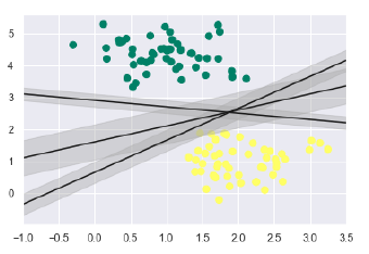
从上面的输出图像中，无涯教程可以轻松地观察到判别式分类器中的"边距"， SVM将选择使边距最大化的线。

链接：https://www.learnfk.comhttps://www.learnfk.com/python-machine-learning/machine-learning-with-python-implementing-svm-in-python.html

来源：LearnFk无涯教程网

接下来，将使用Scikit-Learn的支持向量分类器在此数据上训练SVM模型。在这里，使用线性内核来拟合SVM，如下所示:

from sklearn.svm import SVC # "Support vector classifier"
model = SVC(kernel = 'linear', C = 1E10)
model.fit(X, y)

输出如下-

SVC(C=10000000000.0, cache_size=200, class_weight=None, coef0=0.0,
decision_function_shape='ovr', degree=3, gamma='auto_deprecated',
kernel='linear', max_iter=-1, probability=False, random_state=None,
shrinking=True, tol=0.001, verbose=False)

现在，为了更好地理解，以下内容将绘制2D SVC的决策函数-

def decision_function(model, ax = None, plot_support = True):
   if ax is None:
      ax = plt.gca()
   xlim = ax.get_xlim()
   ylim = ax.get_ylim()

为了判断模型，需要创建网格，如下所示:

x = np.linspace(xlim[0], xlim[1], 30)
y = np.linspace(ylim[0], ylim[1], 30)
Y, X = np.meshgrid(y, x)
xy = np.vstack([X.ravel(), Y.ravel()]).T
P = model.decision_function(xy).reshape(X.shape)

接下来，需要绘制决策边界和边际，如下所示:

ax.contour(X, Y, P, colors='k', levels=[-1, 0, 1], alpha=0.5, linestyles=['--', '-', '--'])

现在，类似地绘制支持向量，如下所示:

if plot_support:
   ax.scatter(model.support_vectors_[:, 0],
   model.support_vectors_[:, 1], s=300, linewidth=1, facecolors='none');
ax.set_xlim(xlim)
ax.set_ylim(ylim)

现在，使用此功能来拟合无涯教程的模型，如下所示:

plt.scatter(X[:, 0], X[:, 1], c=y, s=50, cmap='summer')
decision_function(model);

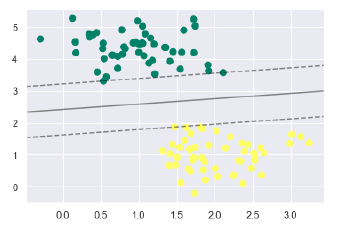
无涯教程可以从上面的输出中观察到SVM分类器适合数据的边距，即虚线和支持向量，该适合度的关键元素与虚线接触。这些支持向量点存储在分类器的 support_vectors _属性中，如下所示-

无涯教程网

model.support_vectors_

输出如下-

array([[0.5323772 , 3.31338909], [2.11114739, 3.57660449], [1.46870582, 1.86947425]])